Proportions
Explanations & examples: For each group; Enter the events (cases) that got the outcome during the time period of the study and enter the total number of people in the group (including the
cases). The proportion (risk) of the cases relative to the total is being calculated for the group together with its 95 % confidence interval. Both the approximated
95 % confidence interval and the exact 95 % confidence interval. The approximated 95 % confidence interval is calculated using the z-distribution (standard normal
distribution) and the exact 95 % confidence interval is calculated using the t-distribution. The latter is more precise, but if the group size is large the two
intervals differ only slightly. The proportion (risk) is a number between 0 and 1. It can be converted into percentage by multiplying with 100 (moving the dot two
steps to the right). The proportion is also converted into odds and the 95 % confidence interval of the odds is shown. For each proportion it can be tested whether it
could be equal, greater than or smaller than a given input value. This is done by entering the value into the field "prop = ... " in the cell "H0". If the p-value here is
below 0.05 the null hypothesis H0 is rejected on a five percent significance level. H0 being that the proportion is either equal to, greater than or smaller than the
input value, depending on your choice in the drop down selector.
For each group; Enter the events (cases) that got the outcome during the time period of the study and enter the total number of people in the group (including the
cases). The proportion (risk) of the cases relative to the total is being calculated for the group together with its 95 % confidence interval. Both the approximated
95 % confidence interval and the exact 95 % confidence interval. The approximated 95 % confidence interval is calculated using the z-distribution (standard normal
distribution) and the exact 95 % confidence interval is calculated using the t-distribution. The latter is more precise, but if the group size is large the two
intervals differ only slightly. The proportion (risk) is a number between 0 and 1. It can be converted into percentage by multiplying with 100 (moving the dot two
steps to the right). The proportion is also converted into odds and the 95 % confidence interval of the odds is shown. For each proportion it can be tested whether it
could be equal, greater than or smaller than a given input value. This is done by entering the value into the field "prop = ... " in the cell "H0". If the p-value here is
below 0.05 the null hypothesis H0 is rejected on a five percent significance level. H0 being that the proportion is either equal to, greater than or smaller than the
input value, depending on your choice in the drop down selector.
For more info about the calculations and formulas used, please see the page medical statistics formulas. If the proportions of at least two groups have been calculated, it can be tested whether the two proportions could be equal in the table "Comparing two proportions". Here, the difference between the proportions is being calculated as well as the ratio (quotient) between them. The ratio of the proportions corresponds to the "relative risk" also known as the "risk ratio", RR. If the null hypothesis H0 to be tested is; the two proportions are the same (there is no statistically significant difference between them) then the value entered in cell null hypothesis is either "difference = 0" or "ratio = 1". If the p-value is under 0.05 then H0 is rejected on a five percent significance level. The weighted estimate (weighted average) of all the proportions entered is also being calculated. The weighted estimate is the common value of the proportion for all groups, combined into one. Taking into consideration the "weight" of each group; a group with more people in it will "weigh" more in the calculation of the weighted estimate and the weighted estimate will therefore lean more towards the "heavier" groups. It is only reasonable to combine all the proportions into one by calculating the weighted estimate if the proportions are not statistically different from each other. It can be tested whether the weighted estimate could be equal to a given other value by entering it into the field "Null hypothesis WE". If p < 0.05 the null hypothesis is rejected on a five percent significance level. Also the crude proportion is being calculated. This is the proportion of all the groups mixed together into one; i.e. all the cases added together divided by all the group totals added together. It can be tested if the crude proportion value can be equal to a certain other value by entering it into the field "Null hypothesis crude". If p < 0.05 the null hypothesis is rejected on a 5 % significance level. Input types: If you already have calculated the no. of cases/events and the total size for each group, then you should choose the default input type "1 × 2 tables". If, on the other hand, you have the data as unanalyzed data in a text file, you should choose input type "raw data". Furthermore; if the data in your text file is in the following format: 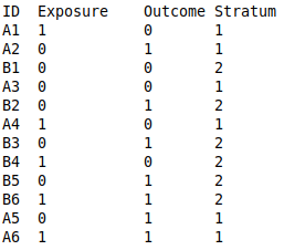 then you should also mark the click option "data in file is in columns" before copy/pasting into the table or reading from a data file. If the data in your text file have the following format; 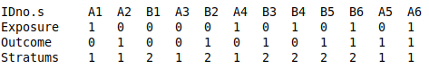 Then you should instead click the check mark "data in file is in rows" before copy/pasting or reading from a data file. Example:If we imagine a fictive, made-up example, where groups were being studied for 8 years divided into the 4 categories of BMI:Group 1: BMI < 18.5 Group 2: 18.5 ≤ BMI < 24.9 Group 3: 25 ≤ BMI < 29.9 Group 4: 30 ≤ BMI We then want to study the connection between high BMI (exposure) and getting a stroke (outcome). The date for the 4 groups being observed is: Group 1: 1 stroke out of 21 people Group 2: 4 strokes out of 89 people Group 3: 13 strokes out of 54 people Group 4: 17 strokes out of 33 people Entered into the tables: 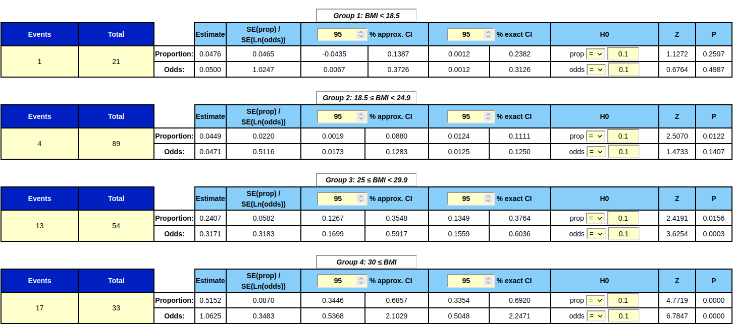 Comparison between group 2 (normal weight) and group 4 (obese): 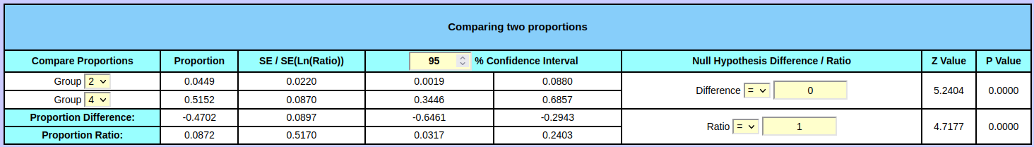 If we for ex. compare the proportions of group 2 and group 4 (namely 0.0449 and 0.5152) it can be seen that the ratio of the two proportions (group 2 relative to group 4) is 0.0872. This ratio is significantly different from 1, since 1 is not included in its 95 % confidence interval going form 0.0317 to 0.2403. Therefore the null hypothesis H0 in this case (the ratio being equal to 1) can be rejected on a five percent significance level. So it does have an effect on the risk of stroke to have a BMI over 30 (obese) compared to have a BMI between 18.5 and 25 (normal weight). Otherwise the two proportions could have been assumed the same. So in this case it wasn't necessary to do the test to see if the proportions could be the same. If you want to do the test anyway, the z-value is 4.7177 and the corresponding p-value is 0.0000, which is far below 0.05. And furthermore: The 95 % confidence intervals of the two proportions in question are [0.0019 : 0.0880] and [0.3446 : 0.6857]. So the confidence intervals don't overlap each other, and therefore the two proportions in question can not be the same and the null hypothesis is (in this case) rejected just by comparing the confidence intervals of the proportions. Similarly; if we compare the proportions of group 2 and 3 we find that they are significantly different from each other. The proportions of group 3 and 4 are also significantly different, as is the case with 1 and 4, but not the proportions of group 1 and 2. Overall considered, the BMI does have an effect on the risk of stroke, in this fictive, made-up example, because the proportions of 4 BMI groups are not the same. So in this case, it isn't recommendable to use or interpret the weighted estimate of all the proportions; since they are pairwise significantly different. |
|
No. of groups:
|
Decimals:
|
|||||||||||||||||||||||||||||||||||||||||||||||||||||||||||||||||||||
|
||||||||||||||||||||||||||||||||||||||||||||||||||||||||||||||||||||||||